CHAPTER 20
Fundamental role of prime numbers and its properties in a complete investigation into Diophantine equations in the sense of existence or non-existent solution and presenting a general solution for the Diophantine equations:
![]()
Some of the generalizations:
![]()
Some of the general generalizations:
![]() ,
, ![]()
20.1. Investigation into extension Fermat’s last theorem 
Before expressing details of Algebraic method of solution of Fermat’s last theorem that Andrew Wiles proved it, we express and solve the general equation:
![]() (1)
(1)
We can study equation (1) in two general forms: ![]() and
and![]() .
.
It is obvious that in case![]() , in fact, we
are face with the Fermat’s last theorem, because:
, in fact, we
are face with the Fermat’s last theorem, because:
![]() ;
;
![]()
With thesis![]() :
:
![]() (2)
(2)
In this section, we try to follow the story of Fermat’s last theorem (famous to Fermat’s great theorem) with reasoning method to acquaint interested persons to mathematics with manner of using Algebraic and geometric methods.
Also, we try to show applications of Wilson’s Euler’s and Fermat’s theorems in solving general equation (1) that is result of researches and continuous attempts of the writer of this book in "20" years and also propounding the last important algebraic results about Fermat’s last theorem that are obtained by the writer.
In this chapter, we follow the history of Fermat’s last theorem till 70s. Importance of this subject is in gathering details of algebraic methods that kummer used it for solving Fermat’s last theorem for the first time. For studying kummer’s works and mathematicians after him that completed his methods, there are a few references except special books. These methods used for many other problems besides attempts to prove Fermat’s last theorem. Therefore, acquaintance with them is useful for interested reader. This part is a sample reference for this purpose. Fermat’s last theorem was proved by Andrew Wiles by using the other mathematician's results after "350" years attempts in 1995. This proof is one of the most important mathematics successes in 20th century in which algebraic methods and geometric methods combined in a beautiful but very complicated manner.
In this brief epilogue that has been written for mathematic interested persons who are not expert in Algebraic geometry, we try to acquaint the reader with some aspects of this proof. Our purpose is only explanation the relation between proof of Fermat’s last theorem and basic guesses in algebraic geometry and therefore, we do not prove the Wiles’s proof. We try only to give a general idea from this part of mathematics. It is clear that exact understanding the Wiles’s proof is not easy and needs to deep study in many years.
20.2. Primitive, Algebraic and geometric methods
Fermat’s last theorem says that if![]() ,
,![]() ,
,
![]() and "
and "![]() "
be integer numbers and we suppose
"
be integer numbers and we suppose ![]() , then at least one of three
numbers
, then at least one of three
numbers ![]() ,
, ![]() and
and ![]() will
be zero. How can we prove such conjecture? Three manners for treating such
problem are natural.
will
be zero. How can we prove such conjecture? Three manners for treating such
problem are natural.
The first method is attempt in using the primitive
methods of number theory. In such attempt, we do not use algebraic
construction, theory of complex numbers and algebraic geometry and we use only
the properties of divisibility of integer numbers. Usual proof of being surd of
![]() is with this method .As we
explained in this book; Fermat himself used these methods for the case of
"
is with this method .As we
explained in this book; Fermat himself used these methods for the case of
"![]() ". These primitive methods
are not easy methods and we can gain many results about Fermat’s last theorem
by using them. But if we adequate only to this methods we can prove only some
special cases of Fermat’s theorem.
". These primitive methods
are not easy methods and we can gain many results about Fermat’s last theorem
by using them. But if we adequate only to this methods we can prove only some
special cases of Fermat’s theorem.
The second method is use of Algebraic methods. This
section explains importance and application of Algebraic methods well and so we
don’t explain it here again. Using these methods, Fermat’s last theorem was
proved for all of integer numbers "n" that![]() .
Although Algebraic methods had important role in Wiles’s proof but they
couldn’t prove Fermat’s last theorem alone.
.
Although Algebraic methods had important role in Wiles’s proof but they
couldn’t prove Fermat’s last theorem alone.
The third method is using the Algebraic geometry. How can we use the geometry to solve a problem like Fermat’s last theorem?
Fermat’s last theorem is an assertion for integer numbers and at least, they haven’t usage in primitive mathematics for solving such problems.
We can show possibility of usage geometric reasoning by an
example. Suppose that we want all of integer numbers which adapt in equation![]() .
With dividing both sides by
.
With dividing both sides by![]() :
:
![]()
If we consider ![]() and
and![]() .
Then the problem is changed to find rational answers of below equation:
.
Then the problem is changed to find rational answers of below equation:
![]()
Every rational answer for this equation is an integer answer
for the first equation and conversely every integer answer of the first
equation (if![]() ) is a rational answer for the
second equation. "
) is a rational answer for the
second equation. "![]() " is equation of circle
centered on origin and with radius of "1". Therefore, we must find
the points on circle that their coordinates be rational numbers.
" is equation of circle
centered on origin and with radius of "1". Therefore, we must find
the points on circle that their coordinates be rational numbers.
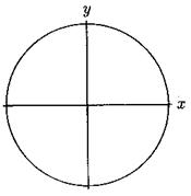
Figure 1.Circle ![]()
With the same method, finding integer answers for equations
like ![]() and other Fermat’s
equations lead to find the points with rational coordinates on a curve in the
plane:
and other Fermat’s
equations lead to find the points with rational coordinates on a curve in the
plane:
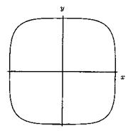
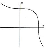
Figure 2. Curves ![]() and
and
![]()
It is interesting that according to Fermat’s last theorem, the first curve (circle) has many points with rational coordinates but on the next curves all of points with rational coordinates have a zero coordinate.
How do we find some points with rational coordinates on a
curve? Solution is easy about a circle. Consider (x, y) as two points on the
circle![]() . Draw the straight line between
point (-1,0) and point (x,y) (we suppose that
. Draw the straight line between
point (-1,0) and point (x,y) (we suppose that ![]() ). We call (o,
t) the place of junction of this line with axes
). We call (o,
t) the place of junction of this line with axes![]() . With
calculation, it seems easily:
. With
calculation, it seems easily:
![]()
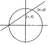
Figure 3. Finding the points with rational
coordinates on curve ![]()
It is resulted that ![]() is a point with
rational coordinates and is on the circle with unit radius if and only if
"t" is a rational number. So if
is a point with
rational coordinates and is on the circle with unit radius if and only if
"t" is a rational number. So if ![]() and
"a" and "b" is integer numbers, then:
and
"a" and "b" is integer numbers, then:
![]() (1)
(1)
So, for finding a point on a circle with rational
coordinates, at first we choose two integer number "a" and
"b" and then by using the formulas (1) we find coordinate of![]() .
Except the point
.
Except the point![]() all of points on circle with
rational coordinate will be obtained. With adding some primitive reasoning, it
is resulted that all of integer answers of equation "
all of points on circle with
rational coordinate will be obtained. With adding some primitive reasoning, it
is resulted that all of integer answers of equation "![]() "
are obtained with below equations:
"
are obtained with below equations:
 (2)
(2)
As we saw, using the geometric concepts for solving the
Fermat’s equation when "![]() ", was very successful. Of
course, we could also use primitive methods of algebraic methods.
", was very successful. Of
course, we could also use primitive methods of algebraic methods.
It is very complicated for "![]() ".
"Faltings" obtained the most successes in this field in 1986. He
proved that many curves like curves "
".
"Faltings" obtained the most successes in this field in 1986. He
proved that many curves like curves "![]() ", have a
limited number of rational point for
", have a
limited number of rational point for![]() . It results
that for every given "n", the number of counter example for
Format’s equation isn’t infinite.
. It results
that for every given "n", the number of counter example for
Format’s equation isn’t infinite.
20.3. An indirect proof of Fermat’s last theorem (elliptic curves)
The method that was useful for proving Fermat’s last theorem
wasn’t one of these direct methods. Of course, Wiles’s proof is based on
algebraic geometry and he used the algebraic method a lot, but this proof,
doesn’t prove Fermat’s last theorem directly. Direct usage of algebraic
geometry means to find the points on curve ![]() with rational
coordinates. Some years before Wiles’s work, other mathematicians arranged new
strategy for solving Fermat’s last theorem. Andrew Wiles concluded this new
method. In the first look, this new method may look a little strange. This
strategy is that we suppose that a counter example exists for Fermat’s last
theorem. So, integer numbers
with rational
coordinates. Some years before Wiles’s work, other mathematicians arranged new
strategy for solving Fermat’s last theorem. Andrew Wiles concluded this new
method. In the first look, this new method may look a little strange. This
strategy is that we suppose that a counter example exists for Fermat’s last
theorem. So, integer numbers![]() ,
, ![]() and
and ![]() exists
so that
exists
so that
![]()
And![]() ,
,![]() and
and![]() .
Number "C" is "
.
Number "C" is "![]() " and with
knowing
" and with
knowing ![]() and
and ![]() finding
finding
![]() isn’t difficult. But two
integer numbers
isn’t difficult. But two
integer numbers ![]() and
and ![]() must
be interesting integer numbers. These two integer numbers are counter example
of Fermat’s last theorem and mathematicians are looking for them around 350
years, so these two numbers must have other interesting properties.
must
be interesting integer numbers. These two integer numbers are counter example
of Fermat’s last theorem and mathematicians are looking for them around 350
years, so these two numbers must have other interesting properties.
Of course, this method is similar to shooting a bullet in darkness, but this method led to prove Fermat’s last theorem.
Mathematic element which is used in this strategy is elliptic curve. We express some properties of elliptic curves and then, we express its coherence with Fermat’s last theorem. Wiles’s proof not only proved Fermat’s last theorem but also proved important properties for elliptic curves. Elliptic curves have important role in algebraic geometry and so, information about them can be useful a lot.
20.3.1. Elliptic curves
Every non-singular cubic curve is called as an elliptic curve. Since we don’t need the most general (and the most precise) definitions, we restrict our self to the
curves with below equation:
![]() (1)
(1)
Other third degree equation can be changed to such equation without changing the curve properties.
It is a non-singular cubic curve if in every point has a well defined tangent and so hasn’t node or cusp. For such equations, we have other equivalent definitions for being non-singular like if:
![]()
And if below system of equations is without any answer:
![]()
Then, cubic curve (1) is non- singular (and then is an
elliptic curve).With a little attention, it is resulted from the last
definition that cubic curve (1) is non-singular if below equation have three
different answers![]() [1]:
[1]:
![]() (2)
(2)
For example, the curve "![]() "
and curve "
"
and curve "![]() " are elliptic (figure 4).
Origin of coordinates is a node (the double point) for curve "
" are elliptic (figure 4).
Origin of coordinates is a node (the double point) for curve "![]() " and a cusp (the triplet
point) for curve "
" and a cusp (the triplet
point) for curve "![]() ". So, these two curves
(figure 5) aren’t elliptic.
". So, these two curves
(figure 5) aren’t elliptic.
Briefly, definition of elliptic curve can be presented in algebraic geometry. Elliptic curve is a smooth projective curve of genus "1". In this book, we define elliptic curve as non-singular cubic curve that is illustrated in equation (1).
(a)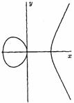 (b)
(b)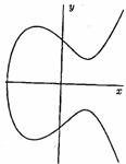
Figure 4. Elliptic curves ![]() (a),
(a),
![]() (b)
(b)
(a) 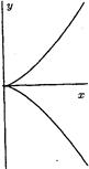 (b)
(b)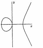
Figure 5. Non-elliptic curves ![]() (a),
(a), ![]() (b)
(b)
Note that we can’t guess only with definition of elliptic curve
that this mathematic element has coherence with Fermat’s last theorem. Of
course Fermat’s equation is an elliptic curve for "![]() ",
namely
",
namely ![]() (as it was mentioned, this
equation that is out of limit of this book, is a cubic curve equation from
equation (1) kind). But Fermat’s equations with higher degree doesn’t form
elliptic curve.
(as it was mentioned, this
equation that is out of limit of this book, is a cubic curve equation from
equation (1) kind). But Fermat’s equations with higher degree doesn’t form
elliptic curve.
As it is said before, this proof uses elliptic curve unexpectedly.
20.3.2. Frey’s elliptic curve and Fermat’s last theorem
Using the primitive reasoning, we can prove that if a counter example exists then a counter example exists too with below conditions:
![]() ,
,![]() and
and ![]() are three integer numbers that
are three integer numbers that
I. ![]() ,
,
II. ![]() ,
,
III. Prime number ![]() exist that
exist that![]() ,
,![]() and
and ![]() are perfect n-th powers,
are perfect n-th powers,
IV. ![]() ,
,![]() and
and ![]() haven’t
a common factor,
haven’t
a common factor,
V. ![]() is
divisible by "32",
is
divisible by "32",
VI. ![]() .
.
VII. ![]() .
.
Gerhard Frey, German mathematician suggested in 1985 that if![]() ,
,![]() and
and ![]() adapt in these conditions,
then we can consider below elliptic curve:
adapt in these conditions,
then we can consider below elliptic curve:
![]() (2)
(2)
Frey thought that it must have very interesting properties.
Note that because of given conditions, equation "![]() "
has three different roots and so equation (2) is a non-singular cubic curve and
in fact it defines on elliptic curve. This elliptic curve is famous as
"Frey’s elliptic curve".
"
has three different roots and so equation (2) is a non-singular cubic curve and
in fact it defines on elliptic curve. This elliptic curve is famous as
"Frey’s elliptic curve".
20.3.3. Why elliptic curve?
Equation (2) is a definition of a special elliptic curve based on a counter example on Fermat’s last theorem. But why we study this elliptic curve? The real reason is that elliptic curves have a lot of properties and because of this a lot of guesses exist about their manner.
Gerhard Frey wasn't looking for solving Fermat’s last theorem. He wanted to find an elliptic curve so that with help of it, he could evaluate some guesses about elliptic curves.
Here we obtain Taniyama- Shimura- Weil conjecture that proving a part of that by Wiles, led to solve the Fermat’s last theorem.
The important point about elliptic curves is that some points with rational coordinates on an elliptic curve form an Abel group! It means that we can define a kind of summation so that when we add two points with rational coordinates on an elliptic curve, the sum will be a point with rational coordinates on that same elliptic curve. More over for this summation we must have a neutral element (zero element) every point with rational coordinates must have inverse and our sum must have property of associativity. It isn’t easy and often it is impossible for non- elliptic curves. Here we show this sum with some example.
For real values, we can draw diagram of elliptic curve in two dimensional
planes. In order to define the summation action on points with rational
coordinates, in the first step, we must add a point to plane. We call this
point as point in infinite and we consider by heart that this point is very for
in ![]() axis. Every straight line
parallel with
axis. Every straight line
parallel with ![]() axis cut this point. More
over, we take in account this point as points with rational coordinates. Adding
this point maybe strange for reader, but in fact, we must consider elliptic
curve in a projective plane for defining the summation and this point is
infinite and in fact, in one of points in infinite of projective plane. For
continuing this subject, exact understanding from projective plane isn’t
necessary and reader can consider the same normal Euclid plane with an
additional point. We show this point in infinite with
axis cut this point. More
over, we take in account this point as points with rational coordinates. Adding
this point maybe strange for reader, but in fact, we must consider elliptic
curve in a projective plane for defining the summation and this point is
infinite and in fact, in one of points in infinite of projective plane. For
continuing this subject, exact understanding from projective plane isn’t
necessary and reader can consider the same normal Euclid plane with an
additional point. We show this point in infinite with![]() .
.
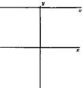
Figure 6. Point in infinite
In figure (7), we have drawn the elliptic curve of![]() . The points
. The points ![]() and
and![]() , are points with rational
coordinates on this curve. Now what is the point
, are points with rational
coordinates on this curve. Now what is the point![]() ? You
may think that we must add coordinates of "P" and "Q"
together, but this action doesn’t give any point on curve. Definition of
? You
may think that we must add coordinates of "P" and "Q"
together, but this action doesn’t give any point on curve. Definition of ![]() is more complicated and is
formed from two stages. At first, we draw a straight line passes from "P"
and "Q". We can prove that this line crosses the elliptic
curve in a third point with rational coordinates. In our example, this third
point is
is more complicated and is
formed from two stages. At first, we draw a straight line passes from "P"
and "Q". We can prove that this line crosses the elliptic
curve in a third point with rational coordinates. In our example, this third
point is![]() . Now, we draw a line parallel to
. Now, we draw a line parallel to ![]() axis from
this third point (in fact, this line joins the third point to a point in
infinite). Since diagram of elliptic curve is symmetric in relation to
axis from
this third point (in fact, this line joins the third point to a point in
infinite). Since diagram of elliptic curve is symmetric in relation to ![]() axis, this line cuts
elliptic curve in a forth point with rational coordinates. In our example, this
forth point is
axis, this line cuts
elliptic curve in a forth point with rational coordinates. In our example, this
forth point is![]() . We call this point
. We call this point![]() , so for curve
, so for curve ![]() we have:
we have:
![]()
Of course we can obtain a formula for this summation, but writing this complicated formula doesn’t help to understand this special summation.
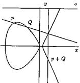
Figure 7. On curve ![]()
We have ![]()
For better understanding, we need to another some examples.
How is the summation of a point with itself? Only difference between this case
and the general case is that we must draw tangent line in the given point,
instead of the first straight line that passed from two points "P"
and "Q". For example in figure (8), on elliptic curve![]() , the point
, the point ![]() is
a point with rational coordinates. Tangent line in this point crosses the curve
in point (4, 12), it means that for this elliptic curve, we have:
is
a point with rational coordinates. Tangent line in this point crosses the curve
in point (4, 12), it means that for this elliptic curve, we have:
![]()
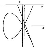
Figure 8. On curve ![]()
We have ![]()
How do we add a point with point "O"? The
first straight line must be vertical and the second line is the same first
line, so, it seems easily that result of summation of every point with point
"O" is the first point itself. In other word, it is neutral in
this summation and plays the role of "zero" .For example, in figure
(9) for elliptic curve![]() , we show:
, we show:
![]()
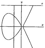
Figure 9. On the curve ![]()
We have ![]()
In figure (10), again we show for elliptic curve ![]() that
that
![]()
In general case, if ![]() is a
point with rational coordinates on the same elliptic curve then
is a
point with rational coordinates on the same elliptic curve then ![]() is also a point with
rational coordinates and more over we have:
is also a point with
rational coordinates and more over we have:
![]()
It means that for defined summation, every member has an inverse.
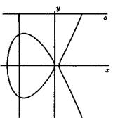
Figure 10. On curve ![]()
We have ![]()
Of course, this point that the points with rational coordinates and with this summand action form an Able group needs to be proved. We hope that the examples which we expressed convince the reader that this isn’t an unexpected assertion.
If ![]() is an elliptic curve,
is an elliptic curve, ![]() is indicator of Abel group
of the points with rational coordinates
is indicator of Abel group
of the points with rational coordinates![]() . Now, we
consider that reader has little information about able groups. Of course, our
immediate purpose is discussion about some properties of
. Now, we
consider that reader has little information about able groups. Of course, our
immediate purpose is discussion about some properties of![]() .
This discussion will convince the reader that information and open problems
about points with rational coordinates on elliptic curves are very much.
Details of this discussion have not so effects on understanding the rest of
this book, so you can ignore them.
.
This discussion will convince the reader that information and open problems
about points with rational coordinates on elliptic curves are very much.
Details of this discussion have not so effects on understanding the rest of
this book, so you can ignore them.
Every Able group like ![]() is direct
sum of the number of cyclic subgroups. Some of these cyclic subgroups are
finite and the others are infinite.
is direct
sum of the number of cyclic subgroups. Some of these cyclic subgroups are
finite and the others are infinite.
We call direct sum of these finite cyclic subgroups as "torsion subgroups" of Able group. Torsion subgroup includes exactly the "elements of finite order". Every infinite cyclic group is "isomorphic" with group of integer numbers.
So, every Able group is direct sum of torsion subgroup and
the number of subgroups that are isomorphic with![]() .
Every cyclic group has a "generator" but the number of generators of
an arbitrary Abel group can be infinite. Mordell proved that the groups
of points with rational coordinates on an elliptic curve can be produced by a
limited number of members. Weil extended this theorem to "number
fields".
.
Every cyclic group has a "generator" but the number of generators of
an arbitrary Abel group can be infinite. Mordell proved that the groups
of points with rational coordinates on an elliptic curve can be produced by a
limited number of members. Weil extended this theorem to "number
fields".
20.3.4. Mordell–Weil theorem
If ![]() is an elliptic curve then
the number of generators of
is an elliptic curve then
the number of generators of ![]() is
finite.
is
finite.
This theorem is important because we can consider some
limits for structure of ![]() without any information
about
without any information
about![]() . It is resulted from what is
said about Able groups and by using the Mordell-Weil theorem that for every
elliptic curve of
. It is resulted from what is
said about Able groups and by using the Mordell-Weil theorem that for every
elliptic curve of![]() :
:
![]()
That ![]() and
and ![]() are
respectively "torsion subgroup" and "rank" of
are
respectively "torsion subgroup" and "rank" of![]() .
.
Knowledge about group ![]() is not
finished to Mordell-Weil theorem. Below deep theorem quotes that every group
can not be the torsion subgroup of this group and it is restricted to only
"15" distinguished groups.
is not
finished to Mordell-Weil theorem. Below deep theorem quotes that every group
can not be the torsion subgroup of this group and it is restricted to only
"15" distinguished groups.
20.3.5. Mazur’s theorem
If ![]() is an elliptic curve and
is an elliptic curve and ![]() is its "torsion
subgroup", then
is its "torsion
subgroup", then ![]() is one of these 15 below
groups:
is one of these 15 below
groups:
![]()
Here, ![]() is indicator of cyclic
group of order "m".
is indicator of cyclic
group of order "m".
Mazur’s theorem is like a miracle. For example, suppose that
you find a point with rational coordinates on an elliptic curve. We call this
point "P". You can find "![]() " by using
the defined summation action. "
" by using
the defined summation action. "![]() ", must be
a point on an elliptic curve and with rational coordinates. With the same
method,
", must be
a point on an elliptic curve and with rational coordinates. With the same
method, ![]() and
and ![]() and
other points from "
and
other points from "![]() " kind that
" kind that ![]() is an integer value are
points with rational coordinates on elliptic curve. Suppose that relation
"
is an integer value are
points with rational coordinates on elliptic curve. Suppose that relation
"![]() " is established for point
"P" .It means that rank of point "P" in group
" is established for point
"P" .It means that rank of point "P" in group
![]() is equal to "7".
It is resulted from Mazur’s theorem that the only points with rational
coordinates and finite rank on elliptic curve are
is equal to "7".
It is resulted from Mazur’s theorem that the only points with rational
coordinates and finite rank on elliptic curve are![]() . If
another point with rational coordinates exists on this curve, then its rank is
infinite. Searching about points with rational coordinates on elliptic curve is
continued. Two open questions that their answers haven’t been found yet in this
book are:
. If
another point with rational coordinates exists on this curve, then its rank is
infinite. Searching about points with rational coordinates on elliptic curve is
continued. Two open questions that their answers haven’t been found yet in this
book are:
1) Can![]() , the rank of "
, the rank of "![]() ", be arbitrarily great?
", be arbitrarily great?
2) Is there any practical algorithm for identification of
being zero of![]() ?
?
20.3.6. Elliptic curves and finite fields
Consider ![]() as a
curve. We can that the points with rational coordinates on
as a
curve. We can that the points with rational coordinates on![]() ,
formed an Abel group and we showed this group by
,
formed an Abel group and we showed this group by![]() . As
the same method and with the same previous summation action, we show the points
with real coordinates on
. As
the same method and with the same previous summation action, we show the points
with real coordinates on ![]() that formed an Abel group
with
that formed an Abel group
with![]() . We obtain diagram of members
of
. We obtain diagram of members
of ![]() when drawing
when drawing ![]() curve. Set of rational
numbers
curve. Set of rational
numbers![]() and set of real numbers
and set of real numbers ![]() are examples of fields. In
a field, we have two actions of summation and multiplication and we can add,
multiply, subtract or divide members of field (of course if it isn’t divisible
by zero). Set of complex numbers
are examples of fields. In
a field, we have two actions of summation and multiplication and we can add,
multiply, subtract or divide members of field (of course if it isn’t divisible
by zero). Set of complex numbers ![]() is
another example of a field. Generally, if
is
another example of a field. Generally, if ![]() is
a field and
is
a field and ![]() is an elliptic curve, then
is an elliptic curve, then ![]() forms an Able group. What
is the purpose of
forms an Able group. What
is the purpose of![]() ? Members of
? Members of ![]() are
pairs
are
pairs ![]() so that "a"
and "b" are members of
so that "a"
and "b" are members of ![]() that
adapt in descriptor equation of
that
adapt in descriptor equation of![]() .
.
We explain it with an example. We consider "p"
as a prime number and ![]() as a finite field with
"p" members. Then
as a finite field with
"p" members. Then![]() ; and actions
summation and multiplication are in "mod 7". So in F7:
; and actions
summation and multiplication are in "mod 7". So in F7:
![]()
We suppose elliptic curve ![]() with
below equation:
with
below equation:
![]()
We can show that this elliptic curve has "5"
points with rational coordinates (Note that we have put this condition that
infinite point "O" is in every![]() ):
):
![]()
Every one of these points adapts in equation ![]() and so if we consider them
with
and so if we consider them
with![]() , we obtain points in
, we obtain points in![]() .
.
Attend that in "![]() " we have
" we have ![]() and so:
and so:
![]()
Of course, it seems directly that every one of these points
adapts in equation![]() . For example, if we put point
. For example, if we put point ![]() in equation
in equation![]() :
:
![]()
That is correct with![]() .
.
In the other hand ![]() isn’t
limited to these "5" points. We have also
isn’t
limited to these "5" points. We have also![]() ,
because:
,
because:
![]()
This example has "2" results:
1) If ![]() then
then ![]()
2) The number of points ![]() is
limited forcedly. And so, finding
is
limited forcedly. And so, finding ![]() is easy.
is easy.
What is usage of "![]() "?
As we saw at the beginning of this section, finding
"?
As we saw at the beginning of this section, finding ![]() is
used in a lot of cases in number theory but usage of
is
used in a lot of cases in number theory but usage of ![]() isn’t
very clear. In this section of Algebraic geometry, the key question is that can
we obtain information about
isn’t
very clear. In this section of Algebraic geometry, the key question is that can
we obtain information about ![]() with knowing
with knowing
![]() for different "p"?
for different "p"?
For example, if for a prime number "p", we
have![]() , then it results that
, then it results that![]() .
.
But what can we conclude in other cases? This question is
important because finding ![]() is easy but
knowing
is easy but
knowing ![]() has more value. If our
considered equations were from degree "l" or "2" then
Hasse-Minkowski theorem would give the positive answer to our question.
has more value. If our
considered equations were from degree "l" or "2" then
Hasse-Minkowski theorem would give the positive answer to our question.
Here we don’t express this theorem because it isn’t adapted
in cubic equations (and so in case of elliptic curves). In case of elliptic
curves ![]() and
and ![]() may
include a point, except
may
include a point, except ![]() for all prime numbers
"p" when
for all prime numbers
"p" when![]() .
.
But the story doesn’t finish here. There is a deep and
miraculous relation between ![]() and
and![]() . Understanding this relation for
primitive understanding from proving of the Fermat's last theorem is very
important.
. Understanding this relation for
primitive understanding from proving of the Fermat's last theorem is very
important.
20.3.7. The number of members of 
Consider below Elliptic curve:
![]()
We consider "p" as a prime number and we
show the number of members of Able group "![]() "
with "
"
with "![]() ". Since "
". Since "![]() " has only "p"
members, "
" has only "p"
members, "![]() " is an integer number and
finite. Like, for "
" is an integer number and
finite. Like, for "![]() ", reader can see easily:
", reader can see easily:
![]()
And then "![]() ". We
remind that when we say "
". We
remind that when we say "![]() ", it
means that point
", it
means that point ![]() adapts in equation "E".
Of course all of arithmetic actions are done in field
adapts in equation "E".
Of course all of arithmetic actions are done in field ![]() and
with
and
with![]() :
:
![]()
We ask reader to find the members of![]() ,
for at least two prime numbers of "p". It isn’t difficult but
it convinces the reader that summation, multiplication and other actions change
completely when "p" changes and consequently we can’t expect
that any relation between "
,
for at least two prime numbers of "p". It isn’t difficult but
it convinces the reader that summation, multiplication and other actions change
completely when "p" changes and consequently we can’t expect
that any relation between "![]() " and
"
" and
"![]() " exists for two different
prime numbers "p" and "
" exists for two different
prime numbers "p" and "![]() ".
For example, compare members of "
".
For example, compare members of "![]() " which is
given above, with members of "
" which is
given above, with members of "![]() ":
":
![]()
It is difficult to imagine any relation between "![]() " and "
" and "![]() " or between
" or between ![]() and
and![]() .
Of course,
.
Of course, ![]() and it is twice of
and it is twice of ![]() but our target is a
predictable relation
but our target is a
predictable relation
In below table, values of ![]() are
given for odd prime numbers up to "47":
are
given for odd prime numbers up to "47":
|
P |
3 |
5 |
7 |
11 |
13 |
17 |
19 |
23 |
29 |
31 |
37 |
41 |
43 |
47 |
|
Mp |
5 |
5 |
10 |
11 |
10 |
20 |
20 |
25 |
30 |
25 |
35 |
50 |
50 |
40 |
The question is that is there any relation between these numbers? "Taniyama–Shimura–Weil" conjecture answer of this question beautifully. An interesting point about this answer is that its start point is in complex functions theory, namely in analysis. This relation between Algebra and analysis is very deep and unexpectedly. For understanding this conjecture reader must be patient and let us start from an apparently dissertated subject. More over, it isn’t strange that if reader is worried about general relation of this subject to Fermat’s last theorem. Interesting aspect of proof of Fermat’s last theorem is that its key part has no relation to Fermat’s last theorem.
Before every thing, we say that with reasoning it seems that
![]() must have value about
"
must have value about
"![]() ". It is seen from the above
table that approximately for any value of "p" this approximate
value isn’t exact but may be it is acceptable that
". It is seen from the above
table that approximately for any value of "p" this approximate
value isn’t exact but may be it is acceptable that ![]() and
"
and
"![]() " grow together to some
extent.
" grow together to some
extent.
For searching the relation between ![]() and
"
and
"![]() ", we consider some simple cubic
curves. Consider the line
", we consider some simple cubic
curves. Consider the line![]() .
.
The number of members of ![]() is
equal to "p" and every one of these "p"
members can be substituted instead of
is
equal to "p" and every one of these "p"
members can be substituted instead of ![]() and so
"p" point is obtained on the line. Always we take in account
point
and so
"p" point is obtained on the line. Always we take in account
point ![]() as a point on line. Then,
at last "
as a point on line. Then,
at last "![]() " points will exist on every
line of
" points will exist on every
line of![]() . We can express the some
reasoning for some kind of other curves. Like, again for
. We can express the some
reasoning for some kind of other curves. Like, again for![]() ,
consider curve "
,
consider curve "![]() ". We must solve equation
"
". We must solve equation
"![]() " for every value of
" for every value of![]() . This equation has answered
generally that "
. This equation has answered
generally that "![]() " is a quadratic residue in
" is a quadratic residue in![]() . In number theory of primitive,
it is proved that exactly half of numbers
. In number theory of primitive,
it is proved that exactly half of numbers![]() , "
, "![]() " are quadratic residue and
if "
" are quadratic residue and
if "![]() " is a quadratic residue
then equation "
" is a quadratic residue
then equation "![]() " has two answers.
" has two answers.
The equation "![]() " has one
answer and usually we take in account
" has one
answer and usually we take in account ![]() as an
answer. It is results that if values of
as an
answer. It is results that if values of ![]() are
distributed among numbers
are
distributed among numbers![]() ,"
,"![]() "
randomly and uniformly, then the number of points with coordinates in
"
randomly and uniformly, then the number of points with coordinates in ![]() on curve "
on curve "![]() " is equal to "
" is equal to "![]() ". Therefore, for
understanding sequence
". Therefore, for
understanding sequence![]() , we must attend to difference of
, we must attend to difference of
![]() and "
and "![]() ". We call this difference
as "error term" and show it with
". We call this difference
as "error term" and show it with![]() :
:
![]()
Below theorem shows that this "error term" can’t
be more than "![]() ".
".
20.3.8. Hasse-Weil theorem
"E" is an elliptic curve and "p"
is a prime number. Usually ![]() is the
number of members of
is the
number of members of ![]() and"
and"![]() " then:
" then:
![]()
Then for continuing the discussion, we come back to example ![]() and as we promised before,
we will use the analysis of complex functions.
and as we promised before,
we will use the analysis of complex functions.
Consider ![]() and also
below function:
and also
below function:
![]() (3)
(3)
If we show the "complex upper half plane" by "H":
![]()
Definition ![]() includes
multiplication of infinite terms. When we expansion this expression, a power
series of "q" is obtained that in fact is "Fourier series
expansion of
includes
multiplication of infinite terms. When we expansion this expression, a power
series of "q" is obtained that in fact is "Fourier series
expansion of![]() function. Note that if we want
function. Note that if we want ![]() in this expansion, we must
attend to the limited number of terms, because none of terms with "
in this expansion, we must
attend to the limited number of terms, because none of terms with "![]() " has any role in
coefficient of
" has any role in
coefficient of![]() .
.
The question is that what
coherence has this function with our subject? Find Fourier expansion of this
function and if "p" is prime number, then put ![]() equal to coefficient of
equal to coefficient of ![]() in this expansion. Finding
in this expansion. Finding ![]() for small values of "p"
is very easy (calculated by using "Maple software"), and these are in
below table:
for small values of "p"
is very easy (calculated by using "Maple software"), and these are in
below table:
|
|
3 |
5 |
7 |
11 |
13 |
17 |
19 |
23 |
29 |
31 |
37 |
41 |
43 |
47 |
|
|
-1 |
1 |
-2 |
1 |
4 |
-2 |
0 |
-1 |
0 |
7 |
3 |
-8 |
-6 |
8 |
For seeing the importance of these numbers, we write also
"![]() " and "
" and "![]() " in below table:
" in below table:
|
|
3 |
5 |
7 |
11 |
13 |
17 |
19 |
23 |
29 |
31 |
37 |
41 |
43 |
47 |
|
|
5 |
5 |
10 |
11 |
10 |
20 |
20 |
25 |
30 |
25 |
35 |
50 |
50 |
40 |
|
|
-1 |
1 |
-2 |
1 |
4 |
-2 |
0 |
-1 |
0 |
7 |
3 |
-8 |
-6 |
8 |
|
|
4 |
6 |
8 |
12 |
14 |
18 |
20 |
24 |
30 |
32 |
38 |
42 |
44 |
48 |
We see that "![]() " that
" that ![]() is equal to the same error
term. It is results that
is equal to the same error
term. It is results that![]() . In other word, in this special
example, we could find a function that its Fourier expansion coefficients give
error terms exactly. So by using them, we can find the number of members of
. In other word, in this special
example, we could find a function that its Fourier expansion coefficients give
error terms exactly. So by using them, we can find the number of members of ![]() exactly. Of course, we may
calculate
exactly. Of course, we may
calculate ![]() at first and then, we
obtain Fourier expansion by using that. So only interesting point about
function
at first and then, we
obtain Fourier expansion by using that. So only interesting point about
function ![]() is that
is that ![]() decompose
easily. "Taniyama–Shimura-Weil" conjecture says that for every
elliptic curve there is such function and more over, this function has good
analytic properties. In fact,
decompose
easily. "Taniyama–Shimura-Weil" conjecture says that for every
elliptic curve there is such function and more over, this function has good
analytic properties. In fact, ![]() isn’t a
normal function but it is in "modular form".
isn’t a
normal function but it is in "modular form".
Still we need more definitions for understanding
"Taniyama-Shimura-Weil" conjecture and also a modular form and in
another side, since this conjecture expresses an exact relation between elliptic
curves and modular forms; we must express some other definition for elliptic
curves. In fact, for this conjecture, some prime numbers are "good"
prime numbers. So "Taniyama-Shimura-Weil" conjecture says
approximately that if ![]() is an elliptic curve then
modular form of
is an elliptic curve then
modular form of ![]() exists so that coefficients
of Fourier expansion
exists so that coefficients
of Fourier expansion ![]() give error terms for
give error terms for ![]() in which "p" is
a "good" prime.
in which "p" is
a "good" prime.
20.3.9. Prime numbers of good reduction and conductor of an elliptic curve
Consider ![]() as an
elliptic curve and "p" as a prime number. If we reduce
equation coefficients in mod "p", a new curve is obtained that
maybe is singular or non-singular. If it is non-singular, it may have double
point (node) or triplet point (cusp).
as an
elliptic curve and "p" as a prime number. If we reduce
equation coefficients in mod "p", a new curve is obtained that
maybe is singular or non-singular. If it is non-singular, it may have double
point (node) or triplet point (cusp).
So, elliptic curve can be classified in three groups in relative to prime number "p":
1) If ![]() be non-singular with mod
"p", then "p" is a prime number of "good
reduction" for
be non-singular with mod
"p", then "p" is a prime number of "good
reduction" for![]() .
.
2) If it has double point (node) with mod "p",
then "p" is called as prime number of "multiplicative
reduction" for![]() .
.
3) If ![]() has triplet point (cusp)
with mod "p", then "p" is called as prime
number of "additive reduction".
has triplet point (cusp)
with mod "p", then "p" is called as prime
number of "additive reduction".
Prime numbers with multiplicative reduction or additive
reduction are called as prime numbers of "bad reduction". More over,
if ![]() is an elliptic curve and
all of prime numbers be good reduction or with multiplicative reduction, then
is an elliptic curve and
all of prime numbers be good reduction or with multiplicative reduction, then ![]() is called as
"semistable".
is called as
"semistable".
Of course, the above definitions are not very exact. Here
our purpose was that without entering to the details, we obtain a general over
view of classification of prime numbers for elliptic curve![]() .
Another reason for inaccuracy of the above definition is that the configuration
of descriptor equation of
.
Another reason for inaccuracy of the above definition is that the configuration
of descriptor equation of ![]() may
change by changing of linear variable despite
may
change by changing of linear variable despite ![]() properties
hasn't been changed. For example, consider "
properties
hasn't been changed. For example, consider "![]() ".
This equation with
".
This equation with ![]() changes to equation "
changes to equation "![]() " that has triplet point and
is singular, but we put in equation
" that has triplet point and
is singular, but we put in equation![]() ,
, ![]() and
and![]() ,
then equation
,
then equation ![]() will be obtained that with
will be obtained that with ![]() is
"non-singular". A definition that changes with a change of linear
variable can not be very useful. But the problem is raised from inaccuracy of
above definition.
is
"non-singular". A definition that changes with a change of linear
variable can not be very useful. But the problem is raised from inaccuracy of
above definition.
In fact, for every elliptic curve there is a "minimal polynomial" that has minimum possible value for those prime numbers of bad reduction.
Above classification of prime numbers must be used for minimal polynomial of every elliptic curve.
If ![]() is an elliptic curve, then
we define an important number for it. We show this number by
is an elliptic curve, then
we define an important number for it. We show this number by ![]() and call is as
and call is as ![]() "conductor". Here
we don’t express the exact definition of
"conductor". Here
we don’t express the exact definition of ![]() and we
only say:
and we
only say:
![]()
That
set ![]() is all of prime numbers. If
"p" be prime number of good reduction, then
is all of prime numbers. If
"p" be prime number of good reduction, then ![]() and if "p"
be prime number of multiplicative reduction, then "
and if "p"
be prime number of multiplicative reduction, then "![]() ".
If "p" be prime number of additive reduction,
".
If "p" be prime number of additive reduction, ![]() is an integer number
greater than "1". The only deficit in this definition is that we have
not defined accurately
is an integer number
greater than "1". The only deficit in this definition is that we have
not defined accurately ![]() for prime numbers of
additive reduction.
for prime numbers of
additive reduction.
Note that ![]() is
"semistable" if and only if
is
"semistable" if and only if ![]() isn’t
divisible by the second power of a prime number.
isn’t
divisible by the second power of a prime number.
20.3.10. Modular forms
Modular forms have a distinguished position in modern
mathematics and it seems that various phenomenon can be explained by using
them. Here we express only general information. Some times we don’t express all
of details since because of their difficulties, continuing its general subject
will be impossible. ![]() is the "upper
half" of "complex numbers plane".
is the "upper
half" of "complex numbers plane". ![]() is
a positive integer number. Consider below set of matrixes.
is
a positive integer number. Consider below set of matrixes.
![]()
So members of ![]() are "
are "![]() matrixes" that their
entries are integer numbers. Their determinant is "1" and their
bottom left entry is divisible by
matrixes" that their
entries are integer numbers. Their determinant is "1" and their
bottom left entry is divisible by![]() .
.
![]() is a group. Action of this
group is multiplication of Matrix. The important point is that this group
"acts" on
is a group. Action of this
group is multiplication of Matrix. The important point is that this group
"acts" on ![]() . It means that every member of
group
. It means that every member of
group ![]() gives a
"permutation" of
gives a
"permutation" of![]() . In fact if
. In fact if ![]() and
and ![]() ,
then we can define
,
then we can define ![]() by using:
by using:
![]()
It is easy to see![]() and for
and for
![]()
We have![]() . Attend that
in left side of this equation, we combined permutations
. Attend that
in left side of this equation, we combined permutations ![]() and
and
![]() while in right side of equation
we multiplied two members of group
while in right side of equation
we multiplied two members of group ![]() together.
together.
Now consider "holomorphic" functions![]() . If such function has some other
properties except being "holomorphic" then we call it a modular form.
Now we explain necessary properties of a modular form. Attend that as limited
as this descriptor properties, then modular forms have more properties and it
means more accuracy of "Taniyama-Shimura-Weil" conjecture.
. If such function has some other
properties except being "holomorphic" then we call it a modular form.
Now we explain necessary properties of a modular form. Attend that as limited
as this descriptor properties, then modular forms have more properties and it
means more accuracy of "Taniyama-Shimura-Weil" conjecture.
The first condition is that integer numbers ![]() and
and ![]() exists
so that for
exists
so that for
![]() we have:
we have:
![]()
Attend that for every arbitrary![]() ,
matrix
,
matrix ![]() is member of
is member of![]() . If we calculate the above
condition about this member we see that
. If we calculate the above
condition about this member we see that
![]()
It means that ![]() must be a
function with alternative period "1". It is resulted that such
function has Fourier expansion and it can be written in below method:
must be a
function with alternative period "1". It is resulted that such
function has Fourier expansion and it can be written in below method:
![]()
This is Fourier expansion in zero. If we don’t have any
negative power "q" in this expansion and in expansion ![]() in other cusps of
in other cusps of![]() , then we call
, then we call ![]() as modular form of weight
as modular form of weight ![]() at level
at level![]() .
If in this
.
If in this ![]() expansions, all "q"
powers be positive (it means we don’t have power zero) then we call
expansions, all "q"
powers be positive (it means we don’t have power zero) then we call ![]() as a "cusp form".
as a "cusp form".
So, these modular forms are very special and therefore, this conjecture that coefficients of one of these modular forms give a lot of information about our elliptic curve is very interesting and unexpectedly.
The story doesn’t finish here. Set of modular forms of
weight ![]() at level
at level ![]() forms a vector space. On
this vector space a sequence of interesting linear operators exists. Here we
don’t express the definition of these operators and adequate only to their
name. These operators are called as "Hecke operators".
forms a vector space. On
this vector space a sequence of interesting linear operators exists. Here we
don’t express the definition of these operators and adequate only to their
name. These operators are called as "Hecke operators".
If a modular form be "eigenfunction" of all Hecke operators it is called as "eigenform".
We repeat that for our subject, the details of these definitions aren’t very important. Only it is necessary to know that an eigenform is a special kind of a holomorphic function and so finding it during studying elliptic curve is like a miracle. Since eigenforms have a lot of properties, their relation with elliptic curves causes a lot of limits on these curves. One of these limits says that Frey elliptic curve can not exists and so we can not find a counter example for Fermat’s last theorem.
20.4. Taniyama-Shimura-Weil conjecture and Fermat’s last theorem
In 1995, a young Japanese mathematician (Yutaka Taniyama) propounded an interesting and bravely conjecture.
This guess became more accurate by "Goro Shimura" laters. The role of "Weil" is not clear and may be his role is limited according to this conjecture to other mathematicians. In today texts, this conjecture is known as "Taniyama-Shimura-Weil" conjecture. Now we can express this guess with more accuracy by using above definition.
20.4.1. "Taniyama-Shimura-Weil" conjecture
"![]() " is an elliptic curve with
integer coefficients and
" is an elliptic curve with
integer coefficients and ![]() is
is ![]() conductor.
For every prime number of good reduction "p", put
conductor.
For every prime number of good reduction "p", put
![]()
Then modular form ![]() exists so
that
exists so
that
1) ![]() weight is "2",
and
weight is "2",
and
2) ![]() is at level
is at level![]() , and
, and
3) ![]() is a eigenform for Hecke
operators, and
is a eigenform for Hecke
operators, and
4) Fourier expansion ![]() gives
numbers
gives
numbers![]() .
.
Still, we don’t determine coherence of this important conjecture with Fermat’s last theorem. We said before that if Fermat’s last theorem is not correct, we can make an elliptic curve as Frey’s elliptic curve by its counter example.
Frey tried to prove, "Taniyama-Shimura-Weil" conjecture is false about Frey’s elliptic curve. It is resulted that if "Taniyama-Shimura-Weil" conjecture is correct then Frey’s elliptic curve can not exists. Therefore, we can not find a counter example for Fermat’s last theorem. "Jean Pierre Serre" showed that if another conjecture (that we don’t mention it here) be correct, then Frey’s assertion can be proved. American mathematician "Kenneth Ribet" could prove Serre’s conjecture in 1986.
20.5. Frey-Serre-Ribet theorem
Consider that ![]() is a
Frey’s elliptic curve. If we can find a modular form for
is a
Frey’s elliptic curve. If we can find a modular form for ![]() according
to prediction to "Taniyama-Shimura-Weil" conjecture, then we can find
this modular form so that its weight is "2" and at level
"2" and more over this form be a cusp form. Such forms don’t exist!
according
to prediction to "Taniyama-Shimura-Weil" conjecture, then we can find
this modular form so that its weight is "2" and at level
"2" and more over this form be a cusp form. Such forms don’t exist!
20.5.1. Result
If "Taniyama-Shimura-Weil" conjecture be correct then Fermat’s last theorem is also correct.
Here we add this explanation that this solution isn’t the only solution of Fermat's last theorem. In late 80s, some other conjectures also existed besides "Taniyama-Shimura-Weil" conjecture that validity of every one of them led to proof of Fermat’s last theorem. Despite attempts of many experts of mathematician, these other conjectures have not been proved and still it isn’t impossible that one of these gives us a better method for proving Fermat’s last theorem. Of course, at any rate, the first proof (and till now, the only proof) of Fermat’s last theorem is by "Taniyama-Shimura- Weil" conjecture.
Andrew Wiles proved "Taniyama-Shimura-Weil" conjecture for "half stable" elliptic curve and since every Frey’s elliptic curve is half stable Fermat’s last theorem was proved. Of course, Wiles’s primitive proof has an important mistake that it had been corrected by Wiles and Taylor later.
20.6. Wiles and Taylor-Wiles theorem
"Taniyam-Shimura-Weil" conjecture is correct for half stable elliptic curves.
20.6.1. Result
Frey’s curve is half stable and so Fermat’s last theorem is correct!
Here, we didn’t express Wiles's proof. This proof is a difficult and interesting that needs more than 200 pages.
Our purpose was that reader found relation between Wiles theorem and Fermat’s last theorem. In Wiles's proof, Galois's representations are used basically.
At last, we say that study in this mathematic course is continuing now that some years after Wiles’s proof in 1999, "Taniyama-Shimura-Weil" conjecture has been proved for all of elliptic curves (and not only for "half stable" elliptic curves).
For more information about proof of Fermat’s last theorem, refer to index of references.
20.7. Latest achievements and fundamental results concerning Fermat's last theorem and its extension (H.M) [2]
20.7.1. Fermat’s last theorem
Below equation hasn’t positive integer answer for ![]() :
:
![]() (1)
(1)
It is necessary to say that in this section, we suppose that equation (1) has positive integer answer.
Proof. Before proving the assertion, we express a basic and important conclusion about equation (1) that has a great role in proof Fermat’s assertion. This conclusion is extracted from proving "Mordell’s conjecture" by "Gred Faltings" that we mention it here just as conclusion.
20.7.2. Conclusion
The number of answers of equation (1) is finite only for![]() .
.
20.7.2.1. Note. We
mention about the last conclusion (20.7.2) that Mordell’s conjecture was
propounded in 1922 and it is verified from geometric property of equation (1),
namely it is proved for ![]() that rational points on
curve
that rational points on
curve ![]() are limited. Now, we
express proof of conclusion (20.7.2) that is very important with Algebraic
method.
are limited. Now, we
express proof of conclusion (20.7.2) that is very important with Algebraic
method.
Proof of conclusion ("H.M" method)
At first we multiply equation (1) in![]() :
:
![]() (2)
(2)
Equality (2) can be written in below form:
![]() (3)
(3)
Supposing ![]() and
and![]() , we write relation (3) in below
form:
, we write relation (3) in below
form:
![]() (4)
(4)
We suppose common value of equation (4) as ![]() that "p"
is a rational number:
that "p"
is a rational number:
![]() (5)
(5)
Below equation is resulted from system (5):
![]() (6)
(6)
Expression of equation (6) is:
![]() (7)
(7)
It is obvious that since ![]() is
a rational number,
is
a rational number, ![]() must be perfect square:
must be perfect square:
![]()
![]()
Equation (8) shows the necessary condition for solving
equation (1). Namely in order to solving equation (1) for![]() ,
there must be a general answer for
,
there must be a general answer for![]() .
.
We know the general answer of equation (1) for![]() , therefore (according to
(19.5)):
, therefore (according to
(19.5)):
 (9)
(9)
It is resulted from system (9):
![]()
Therefore:
![]() (10)
(10)
According to![]() , it is obvious
that
, it is obvious
that![]() , so equality (10) can be written
in below form:
, so equality (10) can be written
in below form:
![]() (11)
(11)
Since![]() , so we must have:
, so we must have:
![]() (12)
(12)
Substituting equalities (12) in equality (11):
![]() (13)
(13)
It is obvious that if ![]() and
and![]() , "p" value is
rational and if
, "p" value is
rational and if![]() and (even)
and (even)![]() ,
so that be rational "p", we must have:
,
so that be rational "p", we must have:
 (14)
(14)
Here, two possible cases will exist:
I) If![]() ,
, ![]() and
and
![]() are respectively smaller than
are respectively smaller than![]() ,
, ![]() and
and![]() :
:
![]()
It is obvious that by continuing, unlimited Fermat’s
reduction will occur and so equation (1) hasn’t answer except "zero"
and therefore, Fermat’s last theorem is proved for " ![]() ".
".
II) If![]() ,
, ![]() and
and
![]() are respectively greater
than
are respectively greater
than![]() ,
, ![]() and
and![]() :
:
![]()
It is obvious that with continuing, the next equations will be obtained and we will have below inequalities:
![]() (15)
(15)
With mathematical induction it is resulted from inequalities
(15) that equation (1) can not have small answers for![]() ,
and with supposition of existing answer for
,
and with supposition of existing answer for![]() , it
has very great answers and in fact when
, it
has very great answers and in fact when![]() , the number of
answers is limited and infinitely great. Here, conclusion (1) is proved in
Algebra method[3].
, the number of
answers is limited and infinitely great. Here, conclusion (1) is proved in
Algebra method[3].
20.7.2.1. Note. According
to proof of Fermat's last theorem for " "
and "
"
and " " it is obvious that "
 " case happen, so for every
"(odd)
" case happen, so for every
"(odd) " and "(even)
 " also "" case happen, because
procedure of proof is same for every"":
" also "" case happen, because
procedure of proof is same for every"":
20.7.3. Conclusion (H.M)
In general case, equation (1) has property of reducibility to special case of every equation from below equations:
![]() (16)
(16)
For proving assertion (20.7.3), it is enough to write
equation (1) in ![]() form and multiply both
sides of this equation in below expression and then rewrite it in form (16):
form and multiply both
sides of this equation in below expression and then rewrite it in form (16):
![]()
In fact, proof of assertion (20.7.3) is resulted from below equality:
![]() (17)
(17)
This very important theorem is extracted from proof of conclusion (20.7.3).
20.7.4. Theorem (H.M)
If one of the equations (16) hasn't any answer in form (17), then equation (1) will not have answer.
The explicit proof of this theorem is resulted from equality (17), because this equality shows reducibility of equation (1) to equations (16).
Here, another important result is that equation (1) isn’t independent to none of equations (16) about existence or none-existence the answer.
In other word, equation (1) depends on equations (16) about existence or non- existence answer.
Here, it is proved that equation (1) hasn’t independent answer and gains its answers from equations (16).
Also, in general case, below conclusion can be extracted from conclusion (20.7.3).
20.7.5. Conclusion (H.M)
In general case, equation (1) has reducibility property to special case of every below equations:
![]() (18)
(18)
In fact, equation (1) depends on general equations (18) about existence or non-existence answer and hasn’t any independence to infinite equations of (18) about existence or non-existence answer.
An important result that is obtained from theorem (20.7.4) is below theorem.
20.7.6. Theorem (H.M)
Necessary conditions for solving equation (1), is existing at least one answers in form (17) for every one of equations (16).
Important result from theorem (20.7.6) is that the hypothesis of existing answer for equation (1) necessitates existing answer for every one of equations (18). In the other hand, according to equation (8):
![]()
Primitive necessary conditions for solving equation (1) for
every natural![]() , is existing of a series of answers
for equation (1) for
, is existing of a series of answers
for equation (1) for![]() . And according to reducibility
property of equation (1) to equations (18), all of them have a series of
special integer answers for
. And according to reducibility
property of equation (1) to equations (18), all of them have a series of
special integer answers for![]() .
.
20.8. Reducibility law (H.M)
The same power equation with index ![]() is
reducible to equations with index "
is
reducible to equations with index "![]() ".
".
For example, equation (16) is reducible to equations with
index ![]() for
for![]() .
.
Explicit proof of this subject is resulted from below equality:
![]() (19)
(19)
![]() (20)
(20)
To gain the equality (20), it is enough to write equation (19) in form of:
![]()
and multiply the obtained equation in below expression:
![]()
Here, we can prove that if equation (16) has a special answer in forms like (17) or (20), in this special case it is reducible to equation (1). It means that for example, if equation (19) has an answer in below form:
![]() (21)
(21)
By using reducibility law, equation (19) is reducible to
equation (1) that we multiply equation (1) in expression ![]() :
:
![]()
And according to equalities (21), we write recent equation in below form:
![]() (22)
(22)
With the same method, if equation (1) reductions to below equation:
![]() (23)
(23)
Equation (23) must have an answer in below form:
![]() (24)
(24)
If equation (23) has an answer in (24) form, equation (23) reduction to equation(1):
![]()
According to below equalities:
![]()
Recent equation is written in below form:
![]() (25)
(25)
For reducing of equation (16) when![]() ,
it is also enough to multiply equation (1) in "
,
it is also enough to multiply equation (1) in "![]() "
that "
"
that "![]() ".
".
Here, it is proved that hypothesis of existing answer for equation (1) led to an answer in the form of (17) for equations (16).
Also, it is proved that if every one of equations (16) have an answer in (17) form, then they are reducible to a special case of equation (1).
In the other hand, we know that in general case, equation
(1) is reducible to every one of equations (16), therefore, hypothesis of
existing answer for equation (1) for every ![]() ruins
the independence of equations (16) about existing or non-existing answer. Also
it is proved that for
ruins
the independence of equations (16) about existing or non-existing answer. Also
it is proved that for![]() , existing answer for equations
(16) is necessary conditions for solving equation (1). So, Algebraic property
of equation (1) namely its reducibility to every one of equations (16) or (18)
is one of reasons that led to non-existing answer for it.
, existing answer for equations
(16) is necessary conditions for solving equation (1). So, Algebraic property
of equation (1) namely its reducibility to every one of equations (16) or (18)
is one of reasons that led to non-existing answer for it.
So, "Fermat’s last theorem" is proved with "Algebraic" and "geometric" properties of the similar exponents of equation (1) exactly.
20.9. Studying Diophantine equation of n-th order
(similar exponents) (H.M)
![]() (1)
(1)
Here before examination of equation (1), we propound an interesting Diaphontus problem. Euler arranged a series of assertions that are necessary for below hypothesis:
"For natural numbers ![]() and
and
![]() that adapt in condition
that adapt in condition![]() , equation (1) hasn’t answer for
natural numbers
, equation (1) hasn’t answer for
natural numbers ![]() ".
".
It is obvious that when![]() ,
Euler’s hypothesis changes to "Fermat’s last theorem". This special
case of hypothesis shows that how much this problem is difficult.
,
Euler’s hypothesis changes to "Fermat’s last theorem". This special
case of hypothesis shows that how much this problem is difficult.
For ![]() and
and![]() ,
we obtain the assertion of below unsolvable equation:
,
we obtain the assertion of below unsolvable equation:
![]() (2)
(2)
In 1914, Werebrussov propounded proof of Euler's assertion
about unsolvable equation (2). L.E. Dickson mentioned this Werebrussov's work
in his book, but he didn’t point out that Werebrussov's proof is wrong. Only in
1935, w. Padhy attended to this mistake. E. Bell repeated this Werebrussov's
mistake. M. Ward proved validity of Euler’s special assertion up to![]() .
.
Euler's conjecture is wrong for ![]() and
and
![]() because:
because:
![]() (3)
(3)
Also, for ![]() and
and![]() , Euler’s hypothesis is rejected
because L.Lander in June, 27, 1966 found below numeral relation:
, Euler’s hypothesis is rejected
because L.Lander in June, 27, 1966 found below numeral relation:
![]() (4)
(4)
Now, by using the "reducibility law" that having
control over the similar exponents equations (1), we prove that many equations
of (1) have answer for powers![]() , "
, "![]() ",
", ![]() and
and![]() .
.
We saw that we can reduce equation ![]() to
every one of equations (1). Also, we can reduce below general equation to many
equations (1):
to
every one of equations (1). Also, we can reduce below general equation to many
equations (1):
![]() (5)
(5)
Here, we adequate to some examples.
20.9.1. Example
With hypothesis of existing answer for equation![]() , an answer is obtained for
equation (1). For solving the equation (1), at first we consider that an answer
exists in
, an answer is obtained for
equation (1). For solving the equation (1), at first we consider that an answer
exists in ![]() form:
form:
![]()
Now, we write the above numeral relation in ![]() form (or
form (or![]() )
and we multiply both sides of the above numeral relation in below numeral
expression:
)
and we multiply both sides of the above numeral relation in below numeral
expression:
(![]()
(or if we write in ![]() form, we
multiply numeral expression (
form, we
multiply numeral expression (![]() and after
necessary summarizing , we have below numeral equalities:
and after
necessary summarizing , we have below numeral equalities:
(In first case) ![]()
(In second case) ![]()
By comparison equation (1) with every one of last equalities, it is obvious that two series of answer are obtained for it:
(First
answer) ![]()
(Second
answer)![]()
20.9.2. Example
By using an assumptive answer of equation![]() ,
an answer is obtained for below equation:
,
an answer is obtained for below equation:
![]() (2)
(2)
For solving this equation, it is enough to put two answers
of equation ![]() that made from an assumptive
answer of equation
that made from an assumptive
answer of equation ![]() equal to each other
(according to example (20.9.1)):
equal to each other
(according to example (20.9.1)):
![]() (3)
(3)
After comparison equation (2) with numeral relation (3), an answer is obtained in below form:
![]()
20.9.3. Example
Equation ![]() is
solvable by using the assumptive answer of equation:
is
solvable by using the assumptive answer of equation:
![]()
For solving above equation, at first we consider that an
assumptive answer of equation ![]() exists in
exists in
![]() form:
form:
![]()
Now, we write above numeral relation in ![]() form
(or
form
(or ![]() or
or![]() ) and
then multiply both sides of this equality in below expression:
) and
then multiply both sides of this equality in below expression:
![]()
After necessary summarizing, we have below numeral equality:
![]()
By comparison our equation with recent numeral relation, we obtain an answer in below form as the same method, two other answers are obtained):
![]()
20.9.4. Remark
By using the reducibility method, we can solve below equation:
![]()
with an assumptive answer of equation![]() .
.
20.9.5. Example
Below equation has answered for![]() ,
, ![]() and
and![]() :
:
![]() (1)
(1)
It is enough to solve the below equation for![]() ,
, ![]() and
and
![]() :
:
![]() (2)
(2)
At first, we write equation (2) in below form:
![]() (3)
(3)
We multiply both sides of equality (3) in conjugate of the
second side![]() :
:
 (4)
(4)
it is obvious that with reduce equation (2) to a special
case of equation (1) for every natural ![]() , with
hypothesis of existing an answer for equation (2), also, answer exist for
equation (1):
, with
hypothesis of existing an answer for equation (2), also, answer exist for
equation (1):
According to these numeral identities, three answers are obtained for equation (1):
Of course the smallest answer of equation (1) is in below
form![]() :
:
![]()
Also, a numeral answer for equation (1) for ![]() of answer series (I) is in
below form:
of answer series (I) is in
below form:
![]()
After dividing this equality by![]() , we
have the smallest answer of equation (1) for
, we
have the smallest answer of equation (1) for![]() :
:
![]() (5)
(5)
And a numeral answer of equation (1) for ![]() of answer series (1) is
also in below form:
of answer series (1) is
also in below form:
![]()
20.9.6. Attention
In fact, equality (5) is equal to:
![]() or
or ![]()
20.9.7. Example
Below equation has answer for![]() ,
, ![]() ,
, ![]() and
and
![]() :
:
![]() (6)
(6)
For determining an answer of equation (6), it is enough to
solve the equation (2) for![]() ,
, ![]() and
and ![]() :
:
![]()
Since this equation is reducible to special case of equation (6):
![]()
![]() (7)
(7)
According to mentioned numeral identities, there are answers for equation (6) so that one of these answers is in below form:
![]()
Therefore, an answer of equation (6) for![]() ,
,
![]() and
and ![]() will
be obtained by substituting the below values in (7):
will
be obtained by substituting the below values in (7):
For determining an
answer for equation (6), we can use below equation’s answer: ![]() (8)
(8)
Because equation (8) can be reduced to a special case of equation (6):
![]() ;
;
![]() (9)
(9)
Therefore, an answer for equation (6) can be resulted from below numeral identities:
So, an answer of equation (6) for![]() ,
,
![]() and
and ![]() can
be obtained with substituting below values in (9):
can
be obtained with substituting below values in (9):
20.9.8. Extension (H.M)
Here, according to present numeral identities in cases![]() ,
,![]() ,
,![]() and
and ![]() , we
can present an answer for below equations:
, we
can present an answer for below equations:
An answer series of these equations will be obtained with "H.M" reduction method in below form:
a special answer of equation (1) is:
![]()
Two another answers series of these equations (2) will
be obtained with "H.M" reduction method ![]() and
we can obtain the equations answers of (3), (4) and (5).
and
we can obtain the equations answers of (3), (4) and (5).
We will be obtained three another answers series with
changing of![]() ,
,![]() ,
, ![]() and
and ![]() .
.
4) ![]()
We will be obtained two another answers series with changing
of![]() ,
, ![]() and
and![]() .
.
5)![]()
We will be obtained three another answers series with
changing of![]() ,
,![]() ,
, ![]() and
and![]() .
.
20.9.9. Result. Here, we show that solve every same powers equation solving another same powers equations. If exist an answer for below equation:
![]() (1)
(1)
The below equations has answer also![]() :
:
![]() (2)
(2)
If considered an answer of equation (1) in below form, we
will be obtained the ![]() answers with changing
answers with changing![]() ,
,![]() , ...
and
, ...
and![]() :
:
So:
![]()
20.9.10. Example
If![]() , determine a general answer
series of below equation:
, determine a general answer
series of below equation:
![]() (6)
(6)
Solution. It is enough to compare equation (6) with below identity:
![]() (7)
(7)
By comparison equation (6) with identity (7):
![]()
20.9.11. Example
Determine an answer series of below equation:
![]() (8)
(8)
Solution. At first, we determine the smallest common multiple of equation powers:
![]()
According to this point that the smallest common multiple of equation power is number 1384, we can write below identity:
![]() (9)
(9)
By comparison equation (8) with identity (9), an answer series with two arbitrary parameters will obtain for equation (8):
![]()
20.9.12. Example
Determine an answer series of below equation:
![]() (10)
(10)
Solution. At first, we determine the smallest common multiple of equation
powers:
![]()
According to the smallest common multiple of equation powers (555385), we can write below identity:
![]() (11)
(11)
By comparison equation (10) with identity (11), an answer series of equation (10) is obtained with "1384" arbitrary parameters:
![]()
20.10. Solving Diophantine equations having non-similar exponents (multi-equalities) (H.M)
In below general equation, if ![]() are
different numbers, we can present an answer series for it
are
different numbers, we can present an answer series for it![]() :
:
![]() (1)
(1)
For determining a general answer series of equation (1), it is enough to compare it with below identity:
 (2)
(2)
By comparison the equation (1) with identity (2), an answer series with "k" arbitrary parameter is obtained for equation (1):
20.10.1. Example
Determine a general answer series of below equation![]() :
:
![]() (3)
(3)
Solution. For determination a general answer series of equation (3), it is enough to compare it with below identity:
![]() (4)
(4)
By comparing equation (3) with identity (4):
![]()
20.10.2. Example.
If![]() , determine a general answer
series of below equation:
, determine a general answer
series of below equation:
![]() (5)
(5)
Solution. It is enough to compare equation (5) with below identity:
![]()
![]()
20.10.3. Problems
Determine a general answer series of below equations.
![]()
![]()
20.11. Finding an answer for extension of Fermat’s last theorem using the theorems related to prime numbers (H.M)
![]()
![]() (1)
(1)
Before examining the equations like (1), it is necessary that we remind basically theorems related to prime numbers like Fermat’s "small" theorem, Euler’s theorem (an extension of Fermat’s "small" theorem ) and Wilson’s theorem .In order to this purpose, at first , we express the title of theorems.
20.11.1. Fermat’s "small" theorem
If "p" be a prime number and![]() , then:
, then:
![]()
20.11.2. Euler’s theorem
If ![]() then:
then:
![]()
20.11.3. Wilson’s theorem
If "p" be prime number:
![]()
Here, it is enough that we present a simple proof for Euler’s theorem, because two other theorems are special cases of Euler’s theorem.
Proof of Euler’s theorem (2)
If ![]() and we suppose that
and we suppose that ![]() and "n" is
simple pack of residue with module "m" and
and "n" is
simple pack of residue with module "m" and![]() .
It is obvious that numbers
.
It is obvious that numbers ![]() are also
simple packs of residues with module "m", because:
are also
simple packs of residues with module "m", because:
By multiplication of congruencies:
![]()
Since![]() , after necessary summarizing:
, after necessary summarizing:
![]()
20.11.4. Explanation
![]() (Euler’s
(Euler’s ![]() Function): the number of numbers
smaller than "m" that are coprime with "m".
Function): the number of numbers
smaller than "m" that are coprime with "m".
Proof of Fermat’s "small" theorem (1)
It is obvious that if "m" be a prime number like "p", Euler’s theorem changes to special case, namely Fermat’s "small" theorem:
![]()
Proof of Wilson’s theorem (3)
In Fermat’s "small" theorem, we can suppose ![]() or
or ![]() and
"p" is a prime number greater than "2",
and
"p" is a prime number greater than "2",![]() and
and![]() .
.
So, special case of Fermat’s "small" theorem is:
![]() (Leibniz's theorem)
(Leibniz's theorem)
![]() (Wilson's
theorem)
(Wilson's
theorem)
By testing, we find that answer of ![]() and
and ![]() are
external and this is also established for
are
external and this is also established for![]() .
.
20.12. Determining a general answer for equation (H.M)
![]() (1)
(1)
For determining an answer series of equation, at first, we calculate an answer series for below equation:
![]() (2)
(2)
For determining an answer series for equation (2), it is enough to compare it
with below "H.M" identity:
![]() (3)
(3)
By comparison equation (2) and identity (3):

Here, if![]() , equation (2)
changes to below equation:
, equation (2)
changes to below equation:
![]() (4)
(4)
(![]() is Euler’s function )
is Euler’s function ) ![]() : The number of natural number
smaller than "n" that are coprime with "n"
for example
: The number of natural number
smaller than "n" that are coprime with "n"
for example ![]() and
and ![]() ,
because 1,5,7, and 11 are coprime with 12.
,
because 1,5,7, and 11 are coprime with 12.
According to Euler’s theorem, if![]() ,
then expression
,
then expression ![]() is divisible by "n",
in the other hand, we can write:
is divisible by "n",
in the other hand, we can write:
 (5)
(5)
(![]() : Integer part of number)
: Integer part of number)
Using relation[4] (5), we write equation (4) in below form:
 (6)
(6)
By comparing equation (1) with identity (6), an answer series of equation (1) is obtained:
 (7)
(7)
20.12.1. Explanation
In equalities (7), if "n" is a prime number like "p"
![]()
And if "m" be a compound number in ![]() form,
form,
(p, q, t,… are prime factors) we can write:
For example:
20.13. Determining a general answer for equation (H.M)
![]() (2)
(2)
Equation (2) is a special case of equation ![]() therefore, for determining
its answer it is enough to choose
therefore, for determining
its answer it is enough to choose![]() or
or ![]() in answer of recent
equation:
in answer of recent
equation:
 (8)
(8)
Answer (8) is a special case of answer (7) for![]() . Of course, answer of equation
(2) is calculable directly. Using Fermat’s "small" theorem and the
same method of solution of equation (1), we can obtain answer (8) for equation
(2).
. Of course, answer of equation
(2) is calculable directly. Using Fermat’s "small" theorem and the
same method of solution of equation (1), we can obtain answer (8) for equation
(2).
20.14. Determining a general answer for equation
(H.M)
(The Fermat-Catalan conjecture  and
the Beal conjecture
and
the Beal conjecture )
)
1.
![]() (Prime number) ,
(Prime number) , ![]() (3)
(3)
For determining an answer series of equation (3), at first we obtain an answer series of below equation:
![]() (4)
(4)
For determining an answer series for equation (4), it is enough to compare it with below "H.M" identity:
![]() (5)
(5)
By comparing equation (4) with identity (5):
 (6)
(6)
Here, if![]() , equation (4)
reduces to below equation:
, equation (4)
reduces to below equation:
![]() (7)
(7)
According to Wilson’s theorem, if "p" be a
prime number, expression ![]() is divisible by "p"
and in the other hand, we can write:
is divisible by "p"
and in the other hand, we can write:
![]() (8)
(8)
(![]() : Integer part of number)
: Integer part of number)
Here, by using the relation (8) and according to condition![]() , equation (7) can be written in
below form:
, equation (7) can be written in
below form:
 (9)
(9)
By comparing equation (3) with identity (9), an answer series of equation (3) will be obtained:
20.14.1. Attention
In above identities and equations, if we convert "p"
to![]() , we obtain the above identities
and answers that always are established for
, we obtain the above identities
and answers that always are established for![]() . (
. (![]() : prime number formula).
: prime number formula).
20.14.2. The Fermat-Catalan conjecture
There are only finitely many triples of coprime integer
powers "![]() " for which
" for which
![]() with
with ![]()
For example:
![]() ,
,
![]() ,
, ![]()
![]() 20.14.3.
The Beal conjecture
20.14.3.
The Beal conjecture
Let "![]() and
and![]() " be positive integers with
" be positive integers with![]() . If
. If ![]() then
then ![]() and
and ![]() have
a common factor..
have
a common factor..
Or, slightly restated:
The equation "![]() " has no
solution in positive integers "
" has no
solution in positive integers "![]() and
and![]() " with "
" with "![]() and
and ![]() "at
least "3" and "
"at
least "3" and "![]() and
and![]() " coprime[5].
" coprime[5].
20.14.4. The "![]() " conjecture
" conjecture
We suppose "![]() " is the
product of the prime divisors of "
" is the
product of the prime divisors of "![]() " with
each divisor counted only once. The "
" with
each divisor counted only once. The "![]() " conjecture
can be formulated as follows:
" conjecture
can be formulated as follows:
For each ![]() , there
is a constant
, there
is a constant ![]() such that if "
such that if "![]() " and "
" and "![]() " relatively prime (or
coprime) and
" relatively prime (or
coprime) and
![]()
Then:
Max![]() .
.
20.14.5. Note.
We can show that if the "![]() " conjecture
holds then there are no solutions to the prize problem when the exponents are
large enough[6].
" conjecture
holds then there are no solutions to the prize problem when the exponents are
large enough[6].
20.15. Determining a general series of answer for Diophantine equations with arbitrary degree by using Wilson's, Fermat's and Euler's theorems and the role of prime numbers formula in arising of Algebraic identities (H.M)
Equation 1:
Prime
numbers ![]()
![]()
Equation 2:
Prime numbers ![]() ,
,
![]()
Equation 3:
![]() ,
, ![]()
20.15.1. Equation
Prime number![]() , Natural
numbers
, Natural
numbers ![]()
![]() ,
, ![]()
For example: ![]()
![]() (
(![]() )
)
According to solution of equation (![]() ),
(20.14) we investigate the extension of this equation and start this section
with below title.
),
(20.14) we investigate the extension of this equation and start this section
with below title.
· Solution
of "p-th" degree equation in below general form and
determining an answer series for it:![]()
![]() (1)
(1)
In equation (1), "p" is a prime number and ![]() are arbitrary rational
numbers and
are arbitrary rational
numbers and![]() .
.
Solution. For solving equation (1), at first we solve below equation and obtain an answer series for it:
![]() (2)
(2)
For solving equation (2), it is enough to compare it with below "H.M" identity:
![]() (3)
(3)
Comparing equation (2) and identity (3):
(4) 
Here, if![]() , then equation
(2) reduces to below equation:
, then equation
(2) reduces to below equation:
![]() (5)
(5)
According to Wilson’s theorem,
if "p" be prime, then expression![]() is
divisible by "p" and in the other hand it is proved that for
every decomposable expression[7]:
is
divisible by "p" and in the other hand it is proved that for
every decomposable expression[7]:
![]() (6)
(6)
(In
relation (5), "p" is a prime number and ![]() is
symbol of integer part of number).
is
symbol of integer part of number).
Now, by using the relation (5) and according to condition: ![]() , equation (4) can be written in
below form
, equation (4) can be written in
below form ![]() :
:
 (7)
(7)
Comparing equation (1) with identity (6), an answer series
of equation (1) will be obtained immediately (in identity (6) we can substitute
![]() (prime numbers formula)
instead of "p", then variable domain will extend to set of
natural numbers (IN), because for every
(prime numbers formula)
instead of "p", then variable domain will extend to set of
natural numbers (IN), because for every ![]() value is prime
):
value is prime
):
(8) 
20.15.1.1. Example
Examine below equation and find a general answer series for it.
![]() (9)
(9)
Solution. It is enough to substitute below values in relations (8):
![]()
Therefore, a general answer series of equation will be obtained:
(A general answer series of equation (9))
(10) 
So, with this answer, equation examination is finished.
20.15.2. Equation
Prime number![]() , Natural
numbers
, Natural
numbers![]() and
and ![]()
![]()
For example. If![]() ,
then:
,
then:
![]()
![]() (II)
(II)
Considering the solution of equation (II) (20.13), we examine the extension of this equation.
Ÿ Solution of n-th degree Diophantine equation in below general form and determining an answer series for it:
![]() (1)
(1)
In equation (1) "p" is a prime number and ![]() are arbitrary rational
numbers and "p" and "m" are coprime namely
are arbitrary rational
numbers and "p" and "m" are coprime namely![]() .
.
Solution. For solving equation (1), at first, we solve below equation and obtain an answer series for it:
![]() (2)
(2)
For determining an answer series for equation (2), it is enough to compare it with below identity "H.M":
![]() (3)
(3)
So:
(4) 
Here, if![]() , equation (2)
changes to below equation:
, equation (2)
changes to below equation:
![]() (5)
(5)
According to Fermat’s (small) theorem, if "p"
is prime number expression "![]() " is
divisible by "p" ("m" and "p"
are coprime), in the other hand we can write:
" is
divisible by "p" ("m" and "p"
are coprime), in the other hand we can write:
 (6)
(6)
(In relation (6), "p" is prime number and ![]() is integer part of number)
is integer part of number)
Now, by using the relation (6), equation (5) can be written in below form:
 (7)
(7)
By comparing equation (1) with identity (7), an answer series of equation (1) is obtained immediately:
(8) 
20.15.2.1. Example
Find an answer series of below equation if![]() .
.
![]() (9)
(9)
Solution method. It is enough to put in relations (8):
![]()
So, an answer series of equation (9) is obtained immediately:
(10) 
20.15.2.2. Result
In special case, if ![]() then:
then:
![]() (11)
(11)
Equation (11), always has answer for every prime number
"p" if![]() . Therefore equation (11) is
indicator of this principle that sum of the same powers of two numbers can be
written as a power of number if powers be coprime.
. Therefore equation (11) is
indicator of this principle that sum of the same powers of two numbers can be
written as a power of number if powers be coprime.
In the other hand, if "m" is not a multiple
of "p" namely![]() , then equation
(11) always has answer, also if
, then equation
(11) always has answer, also if![]() , equation (9)
always has answer.
, equation (9)
always has answer.
20.15.3. Equation
![]() , Natural numbers
, Natural numbers ![]()
![]()
For example. If![]() ,
then:
,
then:
![]()
![]() (
(![]() )
)
Considering the solution of
equation (![]() ) (20.12), examine the extension
of this equation.
) (20.12), examine the extension
of this equation.
Ÿ Solution of Diophantine equation in below general form and determining an answer series for it:
![]() (1)
(1)
In equation (1), ![]() are arbitrary
rational numbers "m" and
are arbitrary
rational numbers "m" and ![]() are
coprime namely
are
coprime namely![]() .
.
Solution. For solving equation (1) and determining an answer series for it, at first, we obtain an answer series of below equation:
![]() (2)
(2)
For determining and answer series for equation (2), it is enough to compare it with below "H.M" identity:
![]() (3)
(3)
By comparing the equation (2) with identity (3):
(4) 
Here, if ![]() equation
(2) reduces to below equation:
equation
(2) reduces to below equation:
![]() (5)
(5)
In equation (5), ![]() is Euler's
function and
is Euler's
function and ![]() is the number of natural
numbers and smaller than "m" that are coprime with it:
is the number of natural
numbers and smaller than "m" that are coprime with it:
Set of number that are coprime with 18 = {17, 13, 11, 7, 5,
1}; ![]() .
.
20.15.3.1. Point
Always attend that number "1" is coprime with all numbers grater than "1".
According to Euler's theorem, if![]() ,
then
,
then ![]() is divisible by "m".
is divisible by "m".
In the other hand, we can write:
![]() (6)
(6)
(In relation (6), "p" is prime number and ![]() is symbol of number integer
part).
is symbol of number integer
part).
Now, by using the relation (6), equation (5) can be written in below form:
 (7)
(7)
By combining the equation (1) with identity (7), an answer series of equation (1) is obtained immediately:
(8) 
20.15.3.2. Attention
If "m" is a prime number like "p",
then ![]() and if "m" is
composite and in
and if "m" is
composite and in ![]() form (that "p",
"q" and "t"…, are prime factors), then always
we can write:
form (that "p",
"q" and "t"…, are prime factors), then always
we can write:
 (9)
(9)
For example. We calculate
![]() for "m=1024",
"m=1025" and "m=1026", from relation (9):
for "m=1024",
"m=1025" and "m=1026", from relation (9):
20.15.3.3. Example
If ![]() ("p" is
prime number) then equation (1) reduces below form:
("p" is
prime number) then equation (1) reduces below form:
![]()
Solution. It is enough in relation (8), we must put ![]() in stead of
in stead of![]() .
.
Abstract of SOLUTION (1)
"H.M" Method
20.15. ![]() . Result
(1)."H.M." theorem
. Result
(1)."H.M." theorem
If:
![]() , Prime number ( p)[8]
, Prime number ( p)[8]
Then below equation has an answer:
![]()
![]()
Proof:
Abstract of Solution (2)
"H.M" Method
20.15.![]() . Result (2) .
"H.M" theorem
. Result (2) .
"H.M" theorem
If:
![]() ,
,
![]() , Prime number (p)[9]
, Prime number (p)[9]
Then below equation has answer:
![]()
Proof:
Abstract of Solution (3)
"H.M" Method
20.15.![]() . Result(3).
"H.M" theorem
. Result(3).
"H.M" theorem
If ![]() then below equation has answer:
then below equation has answer:
![]()
Proof:
![]()
![]() (Euler’s
Function)
(Euler’s
Function)
1. ![]() (Prime number):
(Prime number): ![]()
2. ![]() (Prime
numbers):
(Prime
numbers):
[1]. For more information look at the appendixes I (21.4) in the end of this book.
[2]. All of these conclusions are results of "20" years researches of writer about "Fermat’s last theorem".
[3].
In fact, case (II) is caused from geometry-Algebraic property of equation (1),
namely being limit of rational points on curve![]() .
.
[4]. For more information look at the appendixes I (21.7).
[5] . The prize. Andrew Beal is very generously offering a prize of "$ 5,000" for the solution of this problem. The value of the prize will increase by "$ 5,000" per year up to "$50,000" until it is solved.
[6] .Adapted from: A generalization of Fermat's last theorem, "the Beal conjecture and prize problem"(R. Daniel Mauldin) "mauldin@unt.edu".
[7]. Author proved this subject in a frequently applied theorem in appendixes I (21.5) in the end of this book.
[8]."p"
belongs to set of prime numbers and we can substitute ![]() namely
prime numbers formula instead of it:
namely
prime numbers formula instead of it:
(![]() Domain of new
variable)
Domain of new
variable) ![]()
[9].We
can substitute ![]() instead of
instead of ![]() (
(![]() :
Domain of new variable).
:
Domain of new variable).